You know the feeling: for a project, being it in Azure, AWS or GCP you need to set up some compute instances, and one of the first screens you run into is the overwhelming machine type selection. Hundreds of combinations are possible. After tinkering a few seconds, chances are that you simply use the machine type you selected the previous time. “What can go wrong? It worked last time!” That is what we discover when running into existing infrastructure: often a single ‘favorite’ machine type is chosen for every workload in the project. That can work fine, but it might not be the optimal choice.
It can really pay off to select these types of machines carefully, because that choice will have an effect on both performance and price.
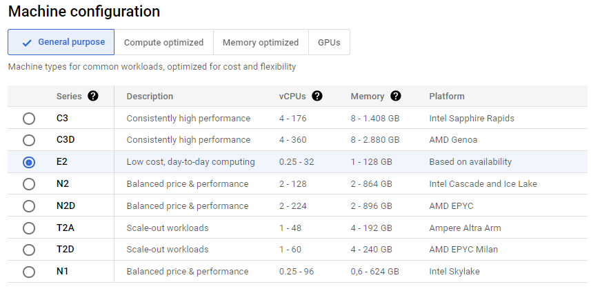
The list of possible compute instance types is overwhelming. E2, N2, N2D, C1, C2, … and all of its subtypes have
- distinct pricing models
- different performance per core
- different cpu/memory commitments
- different commitment price reductions
- …
In the following examples, we made a few assumptions:
- We’re using GCP, although reasoning for Azure and AWS is similar
- Pricing is in US dollars
- Region is EU-west1 (Belgium) (pricing and availability of machine types can be different in other regions)
- The machines are always on. When your application can handle vm interruption on short notice, that will have an effect on your choice too.)
- Pricing is based on the information in the Google Pricing calculator (prices on 2023-12-18)
- We use a free operating system
- The machines used all have 2 cores and 8GB RAM
When it comes to pricing
If costs are your main decision driver, simply comparing the machine types in the Google price calculator is the first thing to do. In the table below, some of the machine types for common workloads (web server, queue processing, …) are compared.
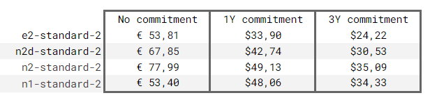
Because of different price reduction schemes, it is clearly visible that the cost reduction is not the same for every machine type. Notably, commitments for N1 machine types are not the best idea, the highest price reduction is only 35% whereas other machine types have up to a 55% price reduction.
But what about the price/performance ratio?
Pricing is one thing, but when performance should be taken in consideration, Google provides some very interesting benchmarks for their machine types to help you: (https://cloud.google.com/compute/docs/coremark-scores-of-vm-instances)
It allow us to make the comparison even more interesting: let’s calculate the Performance per dollar score based on the Coremark benchmark: (higher is better)
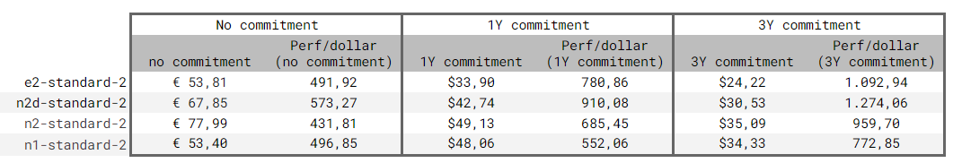
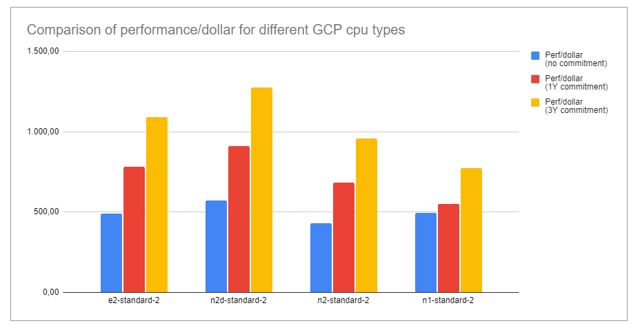
Well, that’s interesting isn’t it? Suddenly n2d pops up as the most interesting choice for common workloads. It gives a stunning 64% more performance per dollar compared to the aging N1 machine type.
Conclusion
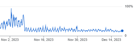
The art of choosing the correct machine type is underestimated. This choice has an enormous impact on pricing and performance. To illustrate this, the chart below of the cpu load of a web server shows what happens when choosing another (better!) machine type with the same amount of cores and memory. The workload was identical before and after the change on the 8th of November. Pricing for this customer only changed with a few dollars/month, but the permanence increase is considerable.
This post is not the end of the story. To keep things readable, we only discussed a subset of the available machine types, and didn’t touch specific workload types (spikes, high performance computing, ARM vs x86, GPU support and performance, OS type ..)
However, we hope these insights can help you make an educated guess on the best machine type for your workload.
And if we can help you make those decisions, feel free to contact us!